Empoower

A poopy library?

Of course, if you dig deep enough like most problems, you'll eventually find your answer. Fortunately, reddit is a very interesting and weird place.

I found the subreddit r/poop which has users submitting their own stool for the judgement of the wider subreddit community. Brilliant - this will work. Not only is there a public forum where users are submitting their stool images, it is also a relatively vibrant community. This is good for how much images I will be able to extract. Stay weird reddit.



Now the problem is, how are we going to extract all of these images? Fortunately, there is a thing called APIs (application programming interface) and reddit so happens to have one. You can access all of the relevant posts made from users in the subreddit community and extract all of the images in high-throughput as most often, the data is stored in JSON files which is very easy to write a script to automate and extract data from. From a couple of subreddits, I was able to extract nearly 2000 images of stool. I now have close to 2000 images of stool. On my laptop. Never have I seen so much in my life. A sample of it is below and I took the liberty of blurring it for viewing pleasure.



Great, we have all of these images so what can we do with them? Well, plenty.

Gain a "deep learning" of your stool

Stool is frankly a goldmine worth of information that continually gets flushed down the toilet. Many scientists like to use it to better understand the microbial residents that live inside of our guts using biochemical and sequencing methods. Yet, sometimes it gets lost that a visual inspection is also a good tool to gain a better glimpse of what's going on inside of our guts.

One tool that can be used to classify stool is based on the bristol stool chart which seperates stool into seven different classes. Often, you will see different frequencies of each class that is associated with gastrointestinal health and diet. One example is that high incidence of type 5 will normally infer a low fiber intake - although I would recommend discussing with a gastroenterologist for best informative information in regards to stool visuals. Below is the bristol stool chart I am referring to.



Fortunately, the field of machine learning has been developed to the point where image classification is no longer as much of a challenging task (although improvements can defintely be made). We can apply this to images of poop. Convolutional neural networks (CNN) is a very powerful algorithim that allows for 'varability' in images to be classified. Computers are inherently logical. This can be a challenge when we want to classify thousand of different images between poop or not poop. Humans have a general idea of what poop looks like and if the poop is in the toilet bowl or on a grassy pile, we as humans can still identify it as poop. Computers on the other hand, won't. Varability in information such as background will be interpreted by computers in a logical method. This is because images are all just data - with pixel values ranging from 0 - 255 in either one channel (gray) or three channels (RGB color system). A grassy background will result in different pixel values from a toilet background. Computers will associate this as different, although there is still a pile of poop in both pictures. Convolutional neural networks helps in differentiating this classification where they take values and size from a select matrix and apply it to an image. This is normally referred to as the kernel. Varying values within that kernel matrix is used to help "identify features" by scaling for specific patterns of the image. And as this kernel parses through the image, a dot product is calculated that will eventually create a convoluted image. An example image below shows the general architecture of convolutional neural networks.



Using this general idea as a platform, I decided to apply the images of stool I have and associate it to whether or not it is poop. I extracted around 1000 images of non-poop related activities and used it to build a convolutional neural network that will tell you whether or not the image is actually poop. Below is a blurred image set as an example.



Using popular deep learning frameworks like tensorflow, I allowed a model to be trained over 14 epochs (or 14 iteration of the dataset) which took approximately four hours to train. It did a reasonable job and can accurately predict whether or not your image is poop with a 95% confidence. Validation loss is also relatively good (lower the better - it is an optimization problem).



Although right now it is only classifying between stool or not stool, my plan is to eventually make it to classify between different types of stool based on something like the bristol stool chart. This will likely be more challenging as building the model requires classifying between seven different types of stool (eight if you are including no stool present). It will also likely require more images and equal distribution between the seven different types of stool. So it becomes a data problem - although there are ways to artifically increase image datasets. I will write about that another time but the biggest bottleneck so far is that I don't want to go through 2000 images and label it between the seven different stool types. It is quite disgusting to look through all those images. Also, I would prefer if a gastroenterologist was with me to better make these educated classifications/labels. It's better to be safer than sorry after all.

A stool's bumpy road in life

Textural analysis is an important tool to better understand how to characterize our droppings. As mentioned prior, different textures in stool usually means something. Therefore, it is important to better learn how to texturally characterize stool and we can use principles from computer vision to do so.

But you may be asking yourself... how can we tell if there is any texture if it is all a flat image? Well, all images is simply a matrix of data and individual pixels are interesting but so are neighboring values of pixels. We can better understand how to segment and texturize an image by looking at when there are sharp changes in pixel values between neighbors and learn the direction of these sharp changes in pixel value differences. This is good because stool has many different types of textures which will make analyses more interesting.

One common way to extract textural properties of an image is by using gabor filters, which is a band-pass filter that only allows specific frequencies to pass through the filter (highlighting for specific patterns in texture). It is essentially a Gaussian that is tuned by a sinusoid. But what exactly does that mean? We will create our own kernel that is made up of frequencies which is then weighted by the gaussian distribution. You can actually see this visibly in the formula below:



Ok - actually maybe it got a bit more confusing. But don't worry it's actually a very easy break down. You can actually see the components of the guassian and the sinusoid. The left exponential function represents the guassian and the right exponential function represents the sinusoid. Below is some images of the probability density function of a guassian and the euler's formula that is related to the sinusoid (whenever you see euler's - you should automatically be thinking circles). The only difference is that this will be in 2-D space rather than 1-D space that we are normally familiar with.

The Guassian Component:

The Sinusoid Component:

All we are basically doing is asking to give a specific size kernel along with a guassian envelope that spans the 2-D kernel space which scales the frequency of the sinusoids - creating interesting filters. And we can change the weights of the kernel by changing the rotation and the axis value (theta) of the guassian. And we can choose to change the sinusoidal part as well. This is what makes gabor filters attractive. You can start seeing how much different filters we can make and how much features we can extract from poop.

With the initial intuition out of the way - let's apply some of this to our image analyses. We will first create a Gabor filter using python and openCV. Our settings will be:

kernel size = (30,30)
sigma = 30
theta = 1/4*pi
lamb = 1/4*pi
gamma = 1
phi = 5

The band-pass filter produced will look something like this:


Let's apply it to a stool image. Even though I blurred these images, you can tell there is quite a bit of textures that is being passed through.

And if we change it to a different direction (90 degrees) and alter the kernel size to (10, 10), we start to see different shapes as well that captures the more vertical component of the textures.

What are some things we can do with this? One of the popular options is to essentially create a bank of filters that is tuned at different angles and etc. And it is quite easy to create a script that modulates all of the different parameters of sigma, theta, lambda, gamma, and phi - put it into a machine learning model to best figure out which set of parameterized values are good filters. This can be quite computationally expensive though depending on how much filters you want to test. You can also do other stuff such as segmentation and quantify specific areas of bumps and the number of bumps in a given stool given we have filters that emphasizes these bump features. These are just exploratory ideas and there is defintely much more you can do if you get creative.

Introducing Mr. Poopy Face

What is the average poop? What drives the differences between poop? Can we reconstruct poop? In facial recognition, a previous common method to gain a sense of someone's face is by understanding the average human face - and how that varies form person to the next. This method is commonly known as eigenfaces where it is possible to break down specific features of a face and how they change across people in general. Before we can create Mr. Poopy Face - we need to first introduce the concept of principal component analyses. It is a very common method for dimensionality reduction which is helpful... cause we can only see three dimensions. PCA is a great tool to use for image analysis to understand your data. PCA is basaically done by assessing the variance of the data set by looking at the direction of spread (eigenvectors) and how much they spread by (eigenvalues).

It is generally a good idea to understand the mathematics behind these operations - especially since it is relatively simple and a good primer for what is ahead. Here are the steps:

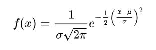
1. Normalize based on normal distribution: (x - mean)/SD
2. Calculate the Covariance Matrix
3. Find the eigenvectors
4. Find the eigenvalues
5. Rank eigenvectors by eigenvalues
6. Project original dataset into the new space of the principal components
7. Plot them

A little explanation.

You standardize the data such that you center everything. This is a good framework to understand how the data moves. You then want to standardize each feature so that all of the variables are on the same paying field. This makes sense when you think of what you are doing when you are trying to find the eigenvectors of a covariance matrix. You are evaluating the amount of variance of how the data moves. And the highest eigenvalues will be associated with the highest variance of the dataset. Now - let's say I have the same exact dataset as my buddy except that I measured something by inches while my buddy measured something with centimeters. We have the same data except his data is scaled by 2.54. So when we look at the variance of that data, his will look to be more signifigant than mine - misleading what is really causing the highest spread of the data.

Now we look into calculating the covariance matrix but first what is it? Well it is the joint varability between two variables. Essentially let's say we have variable x1 and variable x2. When we increase variable x1 - we will ask ourselves - what happens to variable x2? Well if the covariance is greater than 0, then you would expect it to increase with x1. Basically it is correlation without dividing for standard deviation of the population of the data for both x1 and x2. To construct the complete matrix, we do this for the rest of the variables that we have. What will it end up looking like? A symmetric matrix. For simplicity sake, we will just pretend our image just has 3 columns of data as I want to explain how our three columns will produce 3 new eigenvectors that is going to be our new basis. And then we can calculate the covariance matrix just by a simple python command as well.


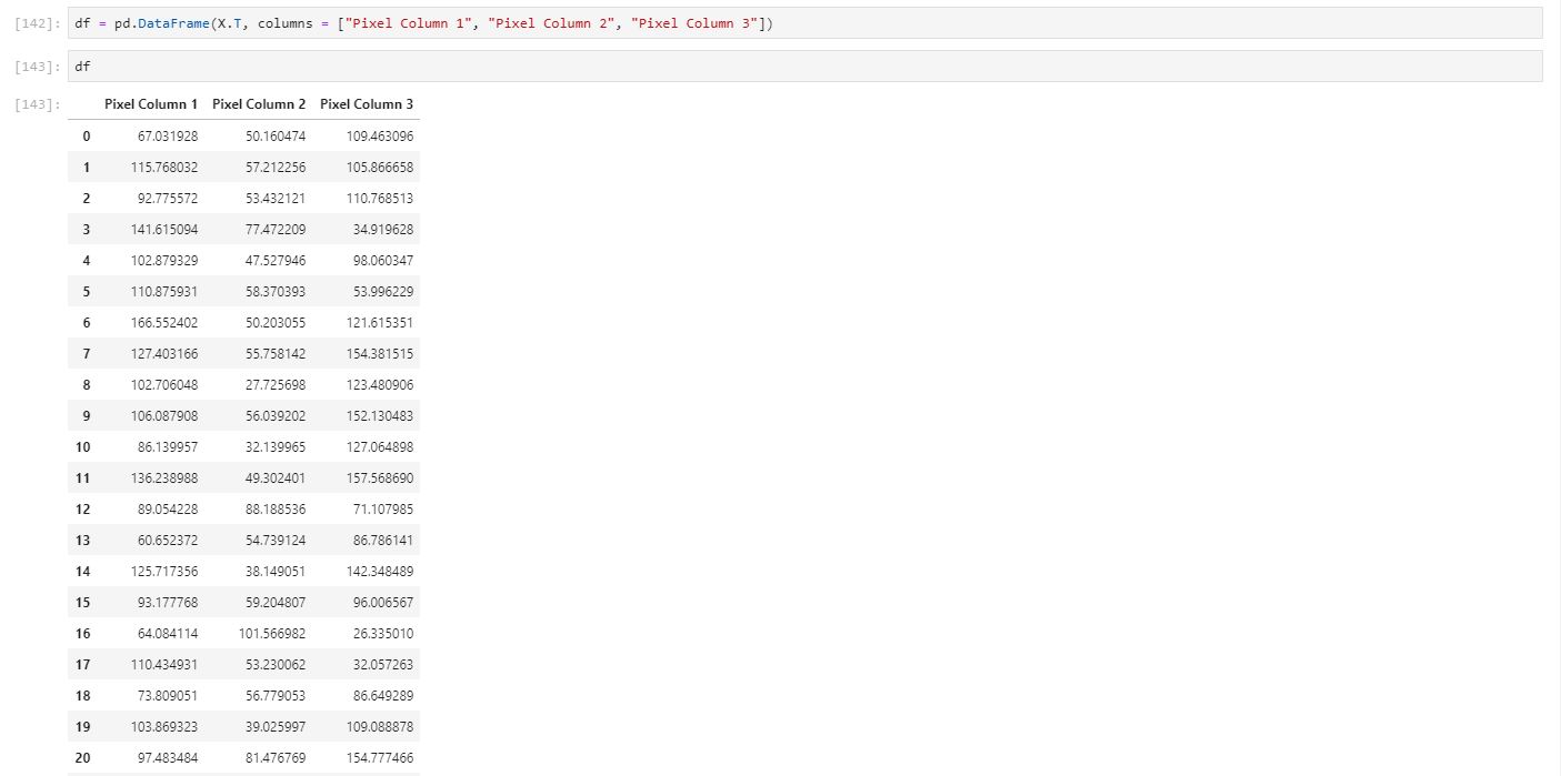
Covariance Matrix:
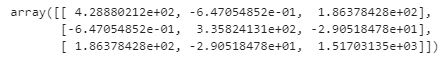
And now we can easily find the eigenvalues and eigenvectors. The number of eigenvectors will be how much variables there were present - if you have 1000 variables, you will have 1000 eigenvectors. In our case, we will only produce three. In most scenarios, calculating it by hand can be labor intensive and pretty unrealistic - especialy if it reaches to 1000 variables. But it is important to kind of understand what is happening here when you try to find the eigenvectors. What we are doing is performing a linear transformation from our original dataset space to another space that explains covariance. When this happens, some of the data will simply be a scalar transformation from our original dataset to the new space. Simply, when we transformed one of the data in our original space, the new transformed data was simply scaled on that specific vector by either 2, -7, and etc. That scalar value is our eigenvalues. And when we look to evaluate the eigenvalues and eigenvectors of the covariance matrix - we are looking at the magntiude of that scalar. Again, for python - it is a simple command and we can calculate our eigenvectors/values from our covariance matrix.

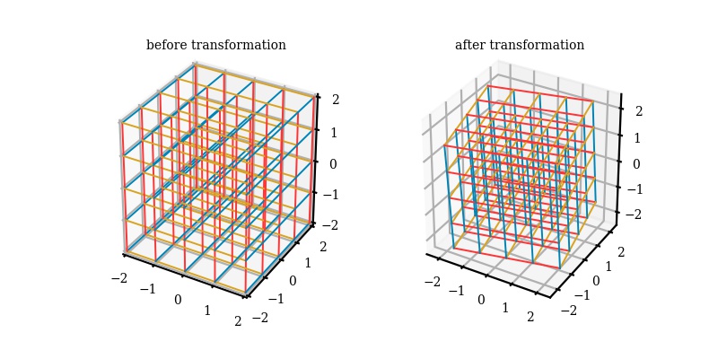
Now we basically have 3 eigenvectors and 3 eigenvalues. We can choose now to rank them from high to low, low to high, or some other way you want to describe the data. It doesn't have to be max eigenvalues! Although that is usually the most popular and usually more useful. So let's say we want to visualize our new data in two dimensions. Easy let's pick our two eigenvectors (based on max eigenvalues) and multiple it to our original dataset subtracted by average mean vector. Now we have transformed our dataset into the space of principal components. In reality, this is simply a change of basis from what we normally consider standard (i component with a unit vector in only the x direction, j component with a unit vector in only the y direction, and k component with a unit vector in only the z direction. I am using a function from a repository made by Barba Lab (https://github.com/engineersCode/EngComp4_landlinear) that quickly shows how after we find our eigenvectors, we can change the basis to the three eigenvectors we have so that we are now in the space of how our data moves in accordance to principal components and from these three - we can reduce the dimension to two (x and y) or one dimension if we so choose.


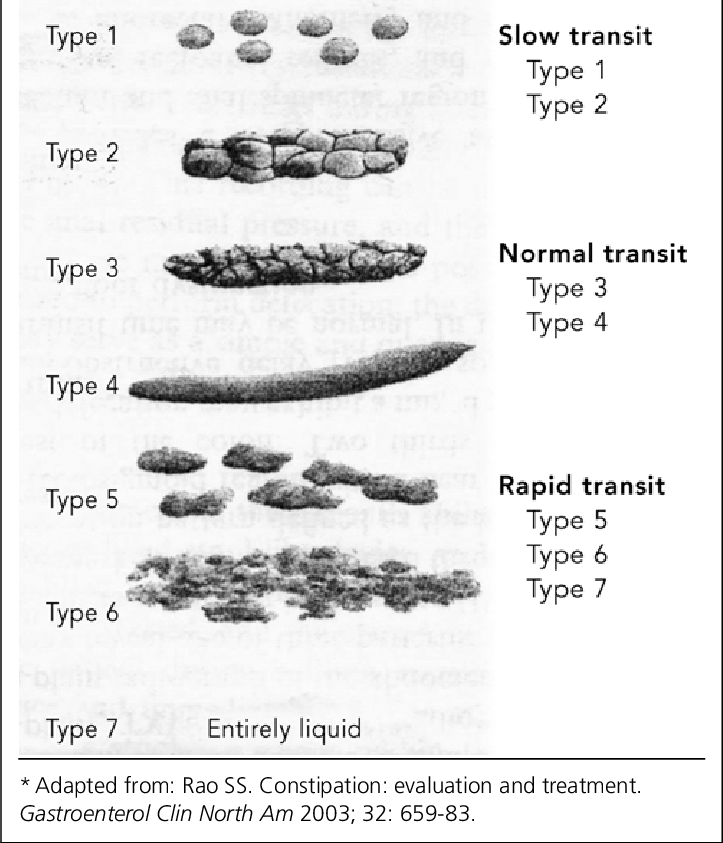
This is all pretty high-level stuff and I would recommend digging through a textbook. I recommend Introduction to Linear Algebra by Gilbert Strang or immersive linear algebra (http://immersivemath.com/ila/index.html) to get a better understanding and nuances you should consider but now to the good part. Once we understood how PCA decomposes our dataset into varability, it is easier to explain why it matters for poop. I kind of gave a primer that poop has different textures and etc but is usually represented by a classification such as the Bristol Stool Chart. What if we take 1000s of images of poop and evaluate the PCA of them? You would essentially get eigenvectors or "modes" where you have the highest variation in data. With this, we can look into classifying stool based on eigenvectors - and let me clarify again, you don't always need to classify based on max variation. Likely the first three with the highest magnitutde might not be a good method to actually classify.


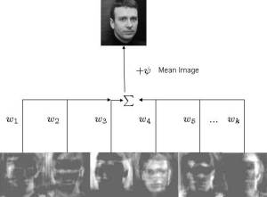
This principle idea is used in some facial recognition algorithims - commonly referred as eigenfaces. In quick summary, we aim to find the "poop" face of specific stool classifications. What is normally done is that you will have an image that is N X N but you will make that image into an N² X 1 vector instead. Once you have this, you can now make a stack of images into a matrix of N² X images. First though, we will resize all of our images to 250 X 250 matrix such that N² will be equal to 62,500 such that this dataset is manageable. I will also only use 20 images as purely an example - and as such our matrix will be 62,500 X 20. Then we calculate a new vector that will be the mean of the 20 images from each pixel value. We subtract each of the 20 image vectors by the mean vector - such that we have centered the data. Once we have that, we can calculate the covariance matrix of this dataset. Usually this is computationally expensive though and single value decomposition (SVD) will be used instead (there are multiple ways to calculate the eigenvectors/values). I won't explain it much in detail but essentially it is another method to decompose our mean subtracted dataset.

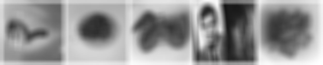
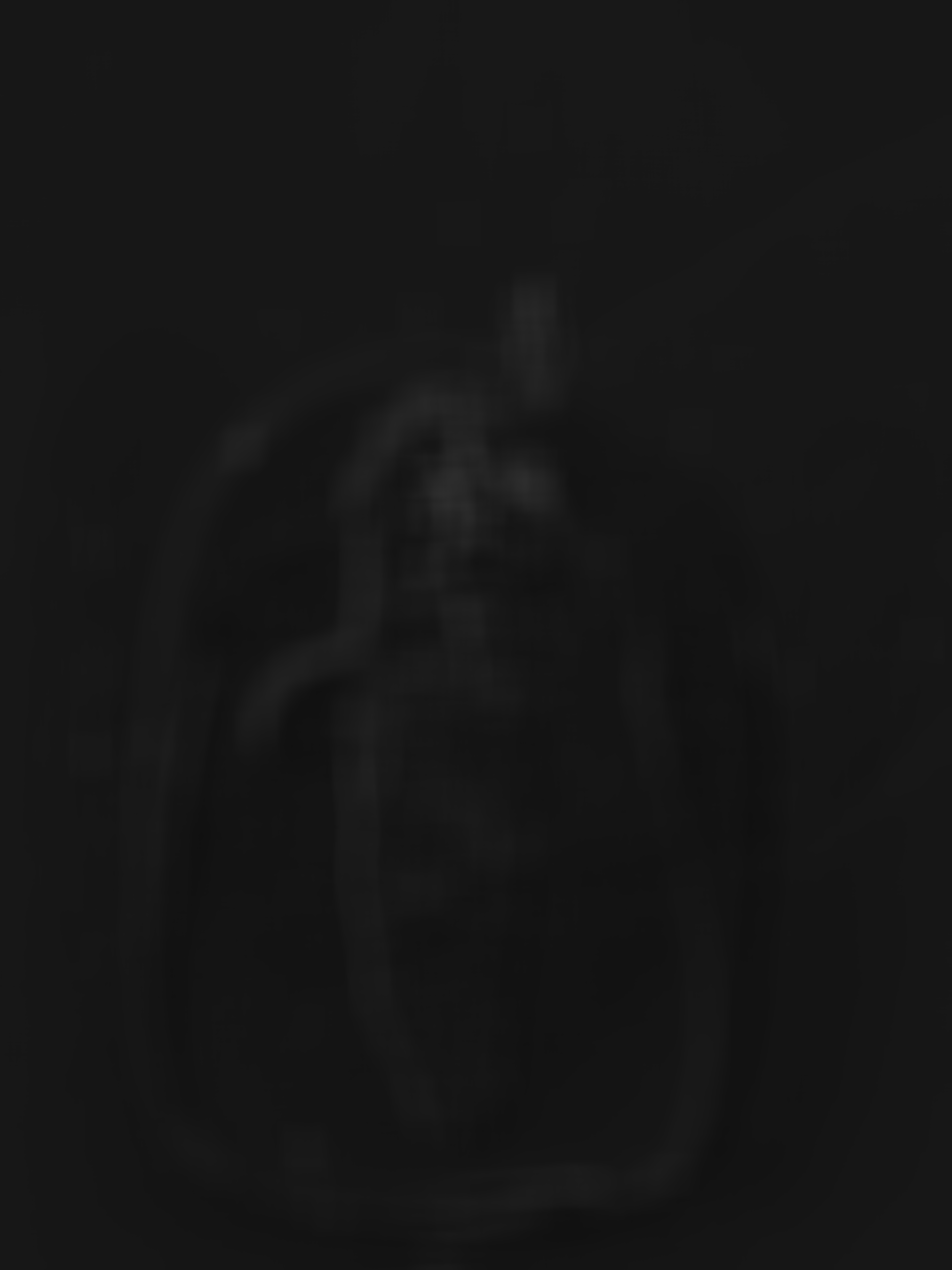
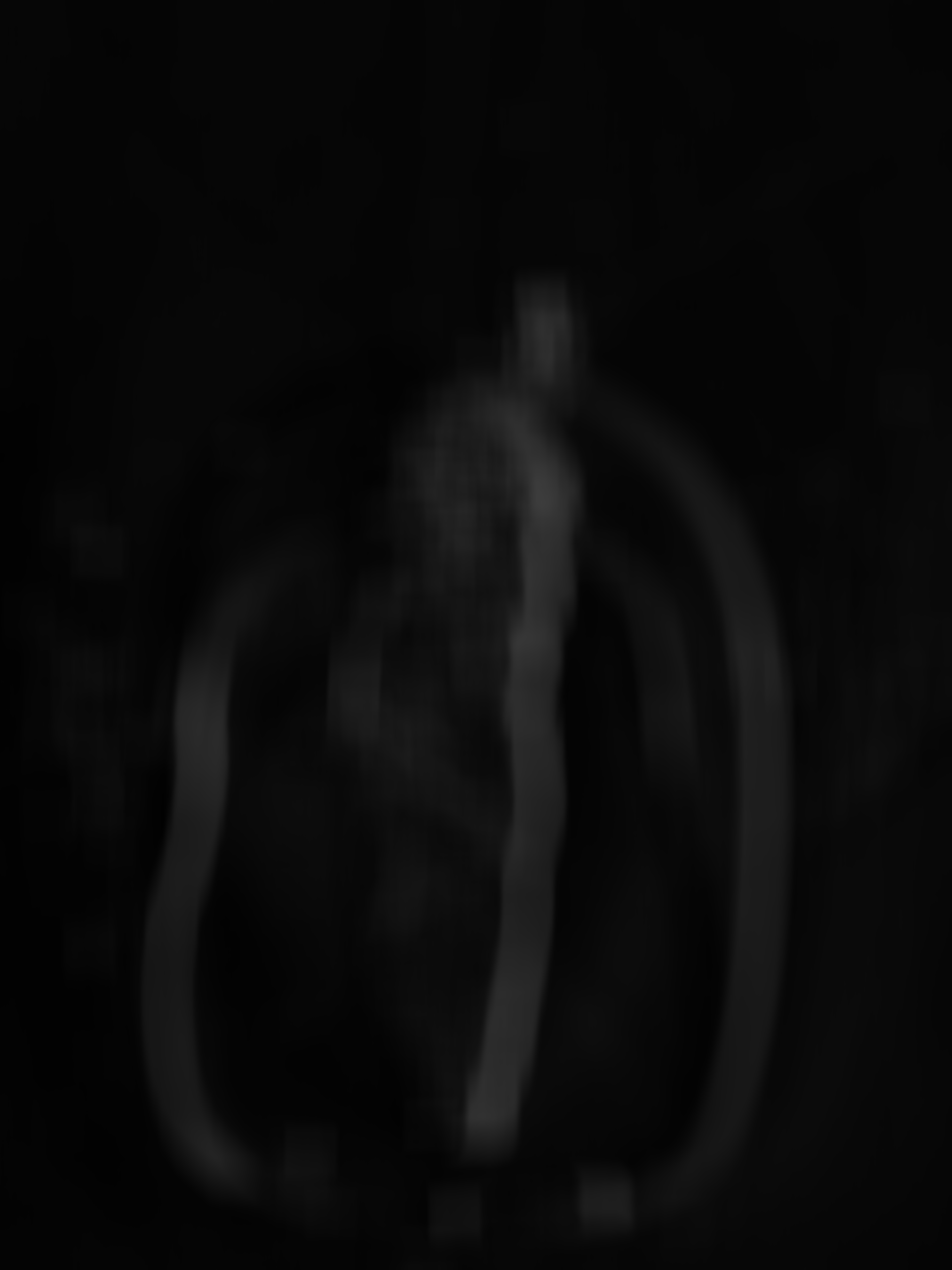
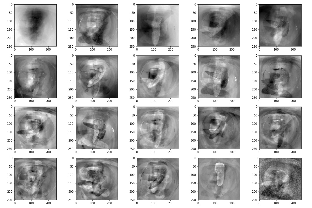
Fortunately, SVD is pretty much a single line code operation with the numpy library and with this we can get our eigenpoops. Below is an image of the mean vector that we had calculated with the eigenvectors that is ordered by eigenvalues or variability based on the covariance matrix. I decided not to blur it this time as it is fairly undistingushable from the daily poo.


Yet, these eigenvectors can be very important and be used to classify different varaitions in the poop images. This could be used as tool to classify more finer details of let's say a bristol stool type 1 classification. Bristol stool is a good option but maybe it could be better? We plan to extend the image analysis capability of stool and this can be an important method to doing so. And I would like to clarify once again that maybe the plotting the eigenvectors associated with highest eigenvalues may not be a good option. Maybe it would be better to look at the 10th ranked eigenvector or the 17th. These eigenvectors may do a better job in classifying variation in bristiol stool type 1s. There are also other opportunities in using these 'eigenpoops' where we can re-construct new stool images. This may be a good to take advantage of in the future if I figure out a good way of applying it to the problem scope but for now, this aim is to find varability with stool classifications.